First steps (Tensorflow)#
In this tutorial we will build small NCP model based on the LTC neuron model and train it on some synthetic sinusoidal data.
pip install seaborn ncps
import numpy as np
import os
from tensorflow import keras
from ncps import wirings
from ncps.tf import LTC
Generating synthetic sinusoidal training data#
import matplotlib.pyplot as plt
import seaborn as sns
N = 48 # Length of the time-series
# Input feature is a sine and a cosine wave
data_x = np.stack(
[np.sin(np.linspace(0, 3 * np.pi, N)), np.cos(np.linspace(0, 3 * np.pi, N))], axis=1
)
data_x = np.expand_dims(data_x, axis=0).astype(np.float32) # Add batch dimension
# Target output is a sine with double the frequency of the input signal
data_y = np.sin(np.linspace(0, 6 * np.pi, N)).reshape([1, N, 1]).astype(np.float32)
print("data_x.shape: ", str(data_x.shape))
print("data_y.shape: ", str(data_y.shape))
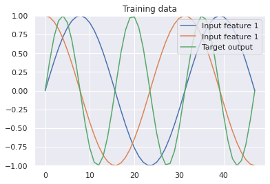
# Let's visualize the training data
sns.set()
plt.figure(figsize=(6, 4))
plt.plot(data_x[0, :, 0], label="Input feature 1")
plt.plot(data_x[0, :, 1], label="Input feature 1")
plt.plot(data_y[0, :, 0], label="Target output")
plt.ylim((-1, 1))
plt.title("Training data")
plt.legend(loc="upper right")
plt.show()
data_x.shape:  (1, 48, 2)
data_y.shape:  (1, 48, 1)
The LTC model with NCP wiring#
The `ncps` package is composed of two main parts:
The LTC model as a
`tf.keras.layers.Layer`RNNAn wiring architecture for the LTC cell above
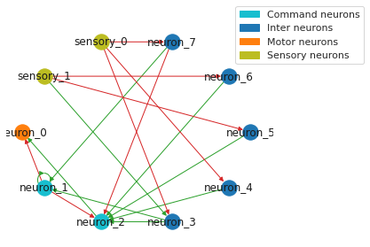
For the wiring we will use the `AutoNCP class, which creates a NCP wiring diagram by providing the total number of neurons and the number of outputs (8 and 1 in our case).
Note
Note that as the LTC model is expressed in the form of a system of [ordinary differential equations in time](https://arxiv.org/abs/2006.04439), any instance of it is inherently a recurrent neural network (RNN). That’s why this simple example considers a sinusoidal time-series.
wiring = wirings.AutoNCP(8,1) # 8 neurons in total, 1 output (motor neuron)
model = keras.models.Sequential(
    [
        keras.layers.InputLayer(input_shape=(None, 2)),
        # here we could potentially add layers before and after the LTC network
        LTC(wiring, return_sequences=True),
    ]
)
model.compile(
    optimizer=keras.optimizers.Adam(0.01), loss='mean_squared_error'
)

model.summary()
Model: "sequential"
_________________________________________________________________
 Layer (type)                Output Shape              Param #
=================================================================
 ltc (LTC)                   (None, None, 1)           350

=================================================================
Total params: 350
Trainable params: 350
Non-trainable params: 0
_________________________________________________________________
Draw the wiring diagram of the network#
sns.set_style("white")
plt.figure(figsize=(6, 4))
legend_handles = wiring.draw_graph(draw_labels=True, neuron_colors={"command": "tab:cyan"})
plt.legend(handles=legend_handles, loc="upper center", bbox_to_anchor=(1, 1))
sns.despine(left=True, bottom=True)
plt.tight_layout()
plt.show()
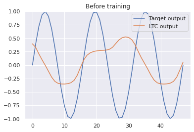
Visualizing the prediction of the network before training#
# Let's visualize how LTC initialy performs before the training
sns.set()
prediction = model(data_x).numpy()
plt.figure(figsize=(6, 4))
plt.plot(data_y[0, :, 0], label="Target output")
plt.plot(prediction[0, :, 0], label="NCP output")
plt.ylim((-1, 1))
plt.title("Before training")
plt.legend(loc="upper right")
plt.show()
Training the model#
# Train the model for 400 epochs (= training steps)
hist = model.fit(x=data_x, y=data_y, batch_size=1, epochs=400,verbose=1)
Epoch 1/400
1/1 [==============================] - 6s 6s/step - loss: 0.4980
Epoch 2/400
1/1 [==============================] - 0s 55ms/step - loss: 0.4797
Epoch 3/400
1/1 [==============================] - 0s 54ms/step - loss: 0.4686
Epoch 4/400
1/1 [==============================] - 0s 57ms/step - loss: 0.4623
Epoch 5/400
....
Epoch 395/400
1/1 [==============================] - 0s 63ms/step - loss: 2.3493e-04
Epoch 396/400
1/1 [==============================] - 0s 57ms/step - loss: 2.3593e-04
Epoch 397/400
1/1 [==============================] - 0s 64ms/step - loss: 2.3607e-04
Epoch 398/400
1/1 [==============================] - 0s 69ms/step - loss: 2.3487e-04
Epoch 399/400
1/1 [==============================] - 0s 73ms/step - loss: 2.3288e-04
Epoch 400/400
1/1 [==============================] - 0s 65ms/step - loss: 2.3024e-04
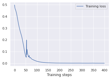
Plotting the training loss and the prediction of the model after training#
# Let's visualize the training loss
sns.set()
plt.figure(figsize=(6, 4))
plt.plot(hist.history["loss"], label="Training loss")
plt.legend(loc="upper right")
plt.xlabel("Training steps")
plt.show()
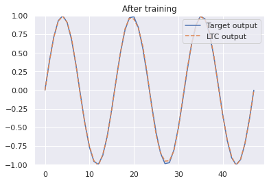
# How does the trained model now fit to the sinusoidal function?
prediction = model(data_x).numpy()
plt.figure(figsize=(6, 4))
plt.plot(data_y[0, :, 0], label="Target output")
plt.plot(prediction[0, :, 0], label="LTC output",linestyle="dashed")
plt.ylim((-1, 1))
plt.legend(loc="upper right")
plt.title("After training")
plt.show()