First steps (Pytorch)#
In this tutorial we will build small NCP model based on the LTC neuron model and train it on some synthetic sinusoidal data.
pip install seaborn ncps torch pytorch-lightning
import numpy as np
import torch.nn as nn
from ncps.wirings import AutoNCP
from ncps.torch import LTC
import pytorch_lightning as pl
import torch
import torch.utils.data as data
Generating synthetic sinusoidal training data#
import matplotlib.pyplot as plt
import seaborn as sns
N = 48 # Length of the time-series
# Input feature is a sine and a cosine wave
data_x = np.stack(
[np.sin(np.linspace(0, 3 * np.pi, N)), np.cos(np.linspace(0, 3 * np.pi, N))], axis=1
)
data_x = np.expand_dims(data_x, axis=0).astype(np.float32) # Add batch dimension
# Target output is a sine with double the frequency of the input signal
data_y = np.sin(np.linspace(0, 6 * np.pi, N)).reshape([1, N, 1]).astype(np.float32)
print("data_x.shape: ", str(data_x.shape))
print("data_y.shape: ", str(data_y.shape))
data_x = torch.Tensor(data_x)
data_y = torch.Tensor(data_y)
dataloader = data.DataLoader(
data.TensorDataset(data_x, data_y), batch_size=1, shuffle=True, num_workers=4
)
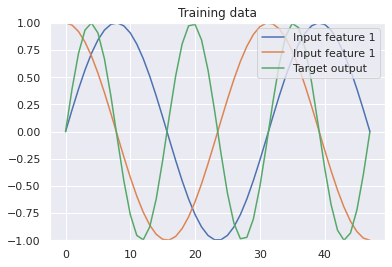
# Let's visualize the training data
sns.set()
plt.figure(figsize=(6, 4))
plt.plot(data_x[0, :, 0], label="Input feature 1")
plt.plot(data_x[0, :, 1], label="Input feature 1")
plt.plot(data_y[0, :, 0], label="Target output")
plt.ylim((-1, 1))
plt.title("Training data")
plt.legend(loc="upper right")
plt.show()
data_x.shape:  (1, 48, 2)
data_y.shape:  (1, 48, 1)
Pytorch-Lightning RNN training module#
For training the model, we will use the pytorch-lightning high-level API. For that reason, we have to define a sequence learning module:
# LightningModule for training a RNNSequence module
class SequenceLearner(pl.LightningModule):
    def __init__(self, model, lr=0.005):
        super().__init__()
        self.model = model
        self.lr = lr

    def training_step(self, batch, batch_idx):
        x, y = batch
        y_hat, _ = self.model.forward(x)
        y_hat = y_hat.view_as(y)
        loss = nn.MSELoss()(y_hat, y)
        self.log("train_loss", loss, prog_bar=True)
        return {"loss": loss}

    def validation_step(self, batch, batch_idx):
        x, y = batch
        y_hat, _ = self.model.forward(x)
        y_hat = y_hat.view_as(y)
        loss = nn.MSELoss()(y_hat, y)

        self.log("val_loss", loss, prog_bar=True)
        return loss

    def test_step(self, batch, batch_idx):
        # Here we just reuse the validation_step for testing
        return self.validation_step(batch, batch_idx)

    def configure_optimizers(self):
        return torch.optim.Adam(self.model.parameters(), lr=self.lr)
The LTC model with NCP wiring#
The `ncps` package is composed of two main parts:
The LTC model as a
`nn.module`objectAn wiring architecture for the LTC cell above
For the wiring we will use the `AutoNCP class, which creates a NCP wiring diagram by providing the total number of neurons and the number of outputs (16 and 1 in our case).
Note
Note that as the LTC model is expressed in the form of a system of [ordinary differential equations in time](https://arxiv.org/abs/2006.04439), any instance of it is inherently a recurrent neural network (RNN). That’s why this simple example considers a sinusoidal time-series.
out_features = 1
in_features = 2

wiring = AutoNCP(16, out_features)  # 16 units, 1 motor neuron

ltc_model = LTC(in_features, wiring, batch_first=True)
learn = SequenceLearner(ltc_model, lr=0.01)
trainer = pl.Trainer(
    logger=pl.loggers.CSVLogger("log"),
    max_epochs=400,
    gradient_clip_val=1,  # Clip gradient to stabilize training
)
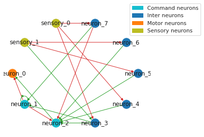
Draw the wiring diagram of the network#
sns.set_style("white")
plt.figure(figsize=(6, 4))
legend_handles = wiring.draw_graph(draw_labels=True, neuron_colors={"command": "tab:cyan"})
plt.legend(handles=legend_handles, loc="upper center", bbox_to_anchor=(1, 1))
sns.despine(left=True, bottom=True)
plt.tight_layout()
plt.show()
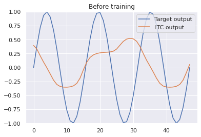
Visualizing the prediction of the network before training#
# Let's visualize how LTC initialy performs before the training
sns.set()
with torch.no_grad():
    prediction = ltc_model(data_x)[0].numpy()
plt.figure(figsize=(6, 4))
plt.plot(data_y[0, :, 0], label="Target output")
plt.plot(prediction[0, :, 0], label="NCP output")
plt.ylim((-1, 1))
plt.title("Before training")
plt.legend(loc="upper right")
plt.show()
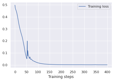
Training the model#
# Train the model for 400 epochs (= training steps)
trainer.fit(learn, dataloader)
.... 1/1 [00:00<00:00, 4.91it/s, loss=0.000459, v_num=0, train_loss=0.000397]
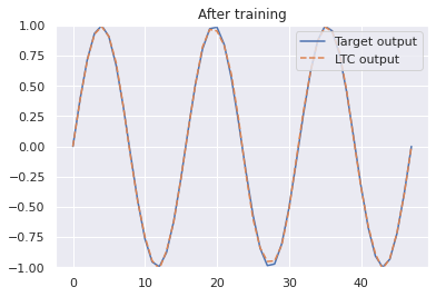
# How does the trained model now fit to the sinusoidal function?
sns.set()
with torch.no_grad():
    prediction = ltc_model(data_x)[0].numpy()
plt.figure(figsize=(6, 4))
plt.plot(data_y[0, :, 0], label="Target output")
plt.plot(prediction[0, :, 0], label="NCP output")
plt.ylim((-1, 1))
plt.title("After training")
plt.legend(loc="upper right")
plt.show()